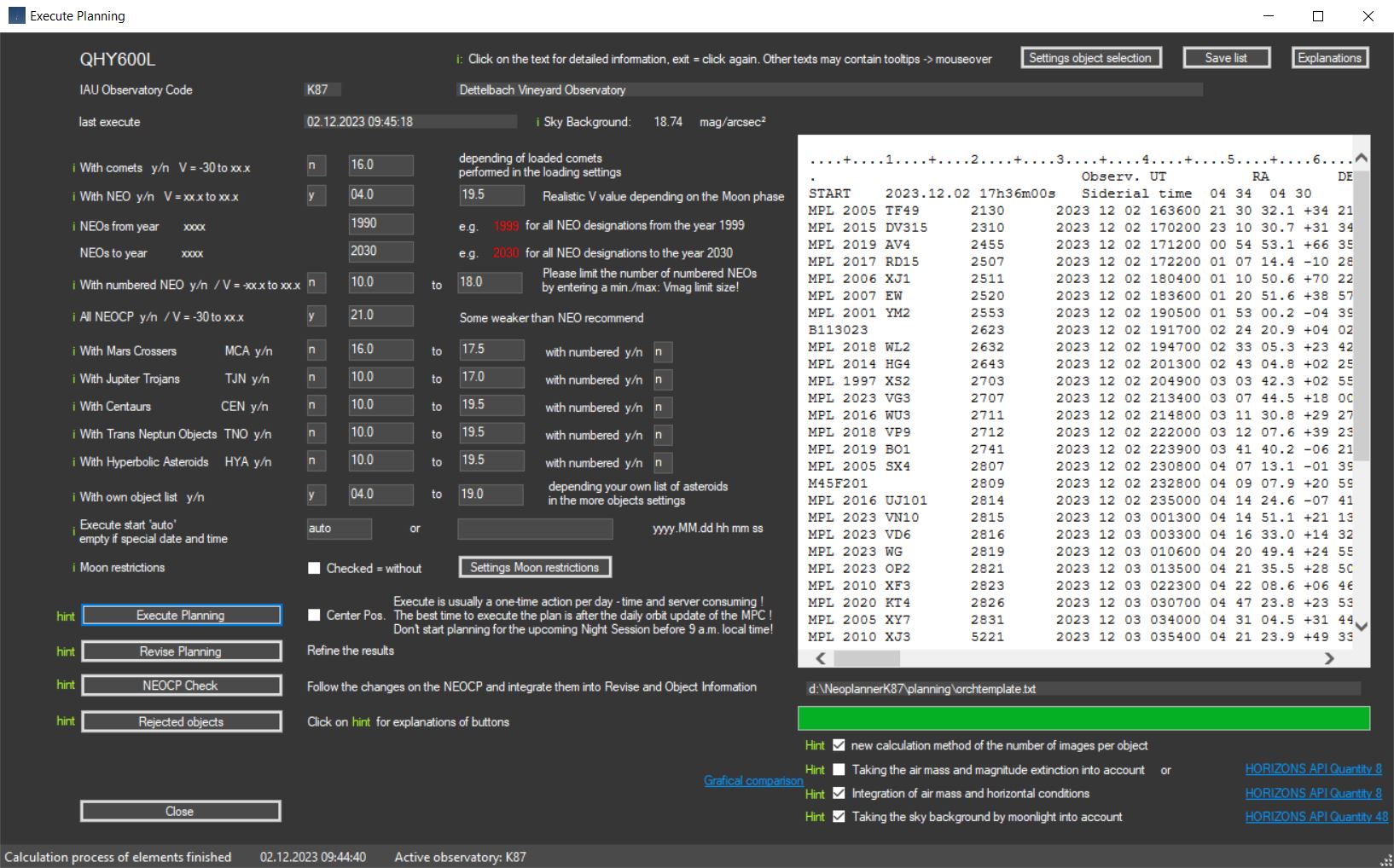
NEO Planner V5.0 - Execute Planning - Explanations
Within the picture, click on the area that you want to be explained: (not in all browsers available)
Origin: The data comes from official access to web services from MPC and Horizons System
Active camera. Clicking takes you to the CCD parameters and you can select the active camera there.
With comets y/n V = -30 to xx.x:
Select here whether you want to include comets in the planning or not. Select the weakest magnitude down to which objects should be considered.
Neo Planner calculates observation times in R.A. order of
currently visible comets according to the official publication of the MPC
and
additionally the most recently observed comets from
CometasObs.
The reason for including the
CometasObs observations lies in the sometimes
considerable delay of the MPC in the publication of the last observations.
More information on the inclusion of comets in the planning process can be found here.
With comets, compared to NEO, you have to apply slightly different standards
with regard to the Vmag selection.
Since comets usually appear spotty on the CCD
image,
the maximum usable brightness should be set somewhat higher than with NEO. In
addition, comets move at far greater distances from the Earth,
which largely excludes a significant change in measured brightness.
29P SCHWASSMANN/WACHMANN with its regularly occurring
outbursts in brightness is certainly an exception here just like
outbreaks in other comets,
but is generally not taken into account.
The real brightness of comets is actually often very different from the
brightness we find in the ephemeris of the MPC.
Therefore to calculate the exposure
times, NEO Planner always uses the average Vmag of the last 10 observations,
which are determined from the last publishing by the MPC
with MPEC XXX: OBSERVATIONS AND ORBITS OF COMETS
AND A / OBJECTS.
With NEO y/n V = -xx.x to xx.x:
Select here whether you want to include NEO the planning or not.
Select the weakest magnitude down to which objects should be considered.
Entering N/n also means that numbered NEO will not be considered. Select the
weakest magnitude down to which objects should be considered.
As a rule, every NEO observer has experience with the maximum NEO observable for
him in relation to their brightness
and should therefore enter his personal
experience value here.
NEO Planner will therefore only select those objects whose Vmag values are
numerically below the settings value.
The apparent speed does not play a role at this point
when considering the maximum usable brightness.
The following model is used to select the NEO:
First it is checked whether the Vmag of the ephemeris
is maximum 0.4 mag weaker than the limit value in the
settings.
If so, the object will continue to be considered.
Second, if the apparent speed in the ephemeris is less
than 100.00 s / min, the average Vmag of the last 10 observations
is used for
the selection of the object,
otherwise the Vmag of the ephemeris.
The reason for taking into account the apparent speed at the time of the
ephemeris is a possible strong
change
in the Vmag compared to previous observations..
At speeds over 100 seconds / minute at the time of the ephemeris
we always use MPC's
designated Vmag of the ephemeris for selection.
Otherwise fast objects might not be taken into account.
In additon, during the calculation of the exposure times,
the selected NEO are subjected to a special Vmag
consideration.
See the explanations for the
revise button in the Preparation / Execute Planning tab
NEO with provisional designations are always included in the planning. Enter the starting year of designations of objects not yet numbered.
These objects have not yet been finally numbered and require
further follow-up observations. Recently discovered NEO,
in particular,
require further observation to improve their orbital elements.
The uncertainty factor U plays a special role in the orbital elements. Objects
with a U factor of 3 or greater
cannot be safely recovered in coming orbits.
U = 0 is the best value.
It is therefore a special and valuable task for amateurs to help improve the
orbital elements of the NEO.
Enter the final year of designations of objects not yet numbered.
With numbered NEO y/n V = xx.x to xx.x:
Select here whether you want to include numbered asteroids
the planning or not. Select the weakest magnitude down
to which objects should be considered.
Numbered objects are not in
the foreground of the observation priorities. However, there may be reasons for
observing objects
whose orbit is very well known.
In the case of numbered NEOs such as 99944 Apophis or other asteroids that are
passing very close to Earth,
there may well be an interest in tracking such NEOs.
In particular, to make meaningful videos for presentation purposes or for other
reasons, it can make perfect sense
also to follow such objects.
In addition, around the full moon there is a good opportunity for diligent
observers to include numbered NEOs
in the list to compensate for the lack of
other objects.
That is why NEO Planner offers the option of including numbered objects in the selection.
The determination of the
observable NEO per observatory code is no longer carried out via the
NEAm00.txt
of the MPC,
but via
the new
API Web Service of the
Horizons system
of the JPL.
This significantly reduces the loading time of the NEO's ephemeris, which is
good for the overall performance of the Execute process.
The loading of all observable numbered NEO of the coming night is now carried
out according to the parameters defined
by NEO Planner such as minimum altitude
or limitation of magnitude.
If numbered objects are selected, please also enter a limit for the magnitude V
here.
All NEOCP object with V = -30 to xx.x:
Confirming NEOCP objects is both a motivation and a challenge. Experience has
shown that observers pay special attention to these objects.
The confirmation of new objects, but also the follow-up observation, is
important in order to allow as many measurements as possible to flow into
the
calculation of the orbital elements for a retrieval in later orbits.
Hint:
The MPC always shows the current positions and
brightness of the objects on the NEOCP.
However, there may be significant fluctuations in brightness at the times
planned with NEO Planner.
It is therefore advisable to enter slightly weaker
brightnesses than usual for NEOCP objects
The following
orbit classes can now also be integrated into the planning.
However, attention should be paid to a narrow selection of brightnesses and not
planned to be mixed with other classes.
Otherwise there is a risk of very long
planning times.
With orbit type Mars Crossers MCA y/n V = xx.x to xx.x with numbered y/n:
Asteroids that cross the orbit
of Mars constrained by (1.3 au < q < 1.666 au; a < 3.2 au).
In order to avoid very long loading times, it is advisable to limit the selected
objects using narrow Vmag from..to entries.
In addition, no other objects should be integrated into the planning.
With orbit type Jupiter Trojans TJN y/n V = xx.x to xx.x with numbered y/n:
Asteroids trapped in the
Lagrange points L4/L5 of Jupiter (4.6 AU < a < 5.5 AU; e < 0.3).
To avoid very long loading times, it is recommended to restrict the selection of
objects by narrow Vmag from..to entries.
Jupiter Trojans are very numerous and mostly already
numbered.
To avoid frustration with the length of time planning or program
crashes this orbit class
should be selected with only unnumbered objects or set the Vmag range very
narrow: e.g. Vmag from 19.0 to Vmag 19.3
In addition, no other objects should be integrated into the planning.
With orbit type Centaur CEN y/n V = xx.x to xx.x with numbered y/n:
Objects with orbits between Jupiter and
Neptune (5.5 au < a < 30.1 au).
In order to
avoid very long loading times, it is advisable to limit the selected objects
using narrow Vmag from..to entries.
In addition, no other objects should be integrated into the planning.
With orbit type TransNeptunian Object TNO y/n V = xx.x to xx.x with numbered y/n:
Objects with orbits outside
Neptune (a > 30.1 au).
In order to avoid very long loading times, it is advisable to limit the selected
objects using narrow Vmag from..to entries.
In addition, no other objects should be integrated into the planning.
With orbit type Hyperbolic <Asteroid> HYA y/n V = xx.x to xx.x with numbered y/n:
<Asteroids> (objects other than comets) on
hyperbolic orbits (e > 1.0).
This orbit class is very rare and should only be of interest when interstellar
objects are newly discovered.
Depending on the interest, the observer can create his
own object list with
any asteroids,
which can be included in the planning selection area.
Application examples are the self-discovered numbered asteroids, which mostly
come from the main belt,
or discovered objects that are not yet numbered.
With the help of this function, a previously popular follow-up list of your own
objects is no longer necessary.
These objects are included in the planning
process and taken into account in the final list,
if the selection was successful according to the settings parameters.
Execute start 'auto', empty of special date and time:
If you enter "auto", the local start time of the planning is determined from the
current GeoSetting data.
First the current sunset and sunrise times are loaded.
Then the offset times from the common restrictions settings are used to
calculate the start and end times.
In the Revise planning display, this data is
displayed as observation slot start and end times.
The calculated start time is used when planning the observation of the first
object. Times can be adjusted in the Revise window.
Always use 'auto' when you call up planning
for the night session.
Adjustments to the start time can then be made in the
Revise Window via the 'Smart Planning' function.
New in version 4.2: To simulate
other observation days, leave the 'auto' field empty
and enter the desired
planning date in local time in the form 'yyyy.MM.dd hh mm ss'.
NEO Planner then calculates the planning data for the date entered. Example:
Simulation of a plan from April 13, 2029, the close flyby of (99942) Apophis, as
shown in the image.
By activating the switch, no moon distance parameters are taken into account in the planning.
Attention: The
planning for the upcoming night session can only be done after 9 a.m. local
time.
All planning before 9 a.m. refers to the previous night session.
You should always plan with >auto<
in Execute Planning. A specific date/time is only intended for simulations.
The time can be adjusted at your own discretion in Revise.
The planning according to the settings and the parameters selected here takes
place in differentiated steps,
which are processed one after the other.
The planning process can be followed in the web browser on the right and in the
progress bar.
First the objects of the current NEOCP are loaded and the observable objects are
selected from them.
Then, together with the observable comets, NEO, numbered and own objects
selected above,
the ephemeris of the coming night session is determined.
After sorting all objects according to R.A. the planning is provided and then
the observation times are calculated according to the settings.
The result of the planning can then be displayed in the Revise and Object
Information Window, edited and, if desired,
made
available on a website.
After the planning has
been completed, interface data like Xml and JSON are created
in the Daily Planning Archive folder,
which in N.I.N.A. can be loaded via the sequencer funktion.
There is also a .txt file release of the planning for the ACP Observatory
Control Software for your own use.
The Execute Planning parameters for the selected camera are saved and reloaded
when the camera is reused.
This means you can now create up to 30 different scenarios in the CCD/CMOS
settings and use them in Execute Planning.
Example: Full moon settings with scenario QHY600L Full Moon period. There are no
limits to the various scenarios, except for the maximum limit of 30.
In the Execute Planning Window you now have the option to choose
between two types of centering objects for the FoV.
a. Centering the object's start position to the center of the FoV (as
before).
b. Centering the middle position of the object path to the center of the
FoV.
By centering on the middle of the object path, you get a much
longer path of fast objects per frame.
The adjusted middle positions are also taken into account in the JSON interface
for N.I.N.A.
and the path is displayed correctly in the Execute Search
window.
In planning is displayed here in the calculated order and provides information
about the objects that can be reached for the coming night.
In addition to the transit time of the object, the observation time calculated
on the basis of the parameters is displayed.
In addition, the planning suggests the exposure times and the number of images
per object.
Here you can also revise and save the planning, e.g. to display it
on a website.
The NEOCP Check function enables the planning to be updated quickly, including
the current NEOCP display.
It is checked whether there are updates for
individual NEOCP objects,
whether these have been deleted or an M.P.E.C. publication
took place.
If new provisional numbers are assigned, these will be determined
and displayed.
Display of rejected objects in
a new window. After every scheduling will update the display.
In the 'Rejected objects' window you can activate rejected objects and start a
new planning there.
New calculation method of the number of images per stack, conceived by Heiko Duin, L65 Bredenkamp Observatory, Bremen:
Switch in the CCD Settings to use a new calculation method for the number of
exposures per object:
The number of images with longer maximum exposure times (e.g. 120
or 180 seconds) and shorter maximum exposure times (e.g. 30 or 15 seconds)
are now calculated correctly. Compared to the previous method, this shortens the
number of images with longer exposure time
and increases the number of shots of slow objects and short exposure time.
Reference values of K87:
href_exposures = 50 Reference value Number of images
href_reso = 3.2 Reference value Resolution FWHM
href_velo = 16.6 Reference value s/min
href_sb = 18.74 Reference value Sky Background SB of NEO Planner
href_mag = 19.4 Reference value Vmag object
href_beltotal = 500 Reference value Total exposure time in seconds for one
measurement
Station values:
sref_reso = resFWHM Station value Resolution FWHM
sref_sb = skybackground Station value Sky Background SB of NEO Planner
sref_maxexp = maxexp Station value maximum exposure time in seconds
Formula Visual Basic:
step1 = sref_reso / velocity(obj) * 60
step2a = href_mag - Vmag(obj)
step2b = href_sb - sref_sb
step2c = step2a - step2b
step3 = 1 / (2.512 ^ step2c)
step4 = href_beltotal * step3
If step1 > sref_maxexp Then
step5 = sref_maxexp
Else
step5 = step1
End If
step6 = CInt(Math.Floor(step4 / step5)) + 1
total number of exposures = step6 * number of
groups
Heiko's method is more elegant and mathematically precise than my old method.
The minimum number of images per stack is 1.
Both methods make it possible to calculate the necessary image sequences
independently of the equipment.
I would like to add one important hint. Objects of the
solar system, regardless of their type,
have different albedos due to their
chemical and physical properties.
So it is perfectly normal that a carbon-rich asteroid is harder to astrometry
than a ferrous one.
The same is true for highly condensed comas in comets as compared to less
strongly condensed comas.
However, NEO Planner cannot know the albedo of the individual objects.
Therefore
everyone has to expect that the observation can go wrong due to
too few images in the stack.
For years I have been observing NEO and comets with my formula and have achieved
useful results.
Both the reference data and the formulas
therefore have a certain practical value, and by no means a scientific
one.
Taking airmass and magnitude extinction into account (scientifically, all objects)
Useful when humidity is low and/or there is little or no light brightening the horizon.
When the checkbox is activated, the relative airmass of the location is taken into
account
when calculating the number of images per group/stack.
The altitude of the object at the time of observation is used.
The consideration of airmass and moon-sky background is only calculated at
altitudes above the minimum value in the Common
Restrictions.
The values used to calculate the airmass come from the JPL HORIZONS API, here
is the description:
_RELATIVE_ optical airmass and magnitude extinction:
Airmass is the ratio of the absolute optical airmass at the targets refracted
elevation angle with the absolute optical airmass at zenith.
Also output is the estimated visual magnitude extinction due to atmosphere, as
seen by the observer. (end of description)
Source: Description
HORIZONS API
Quantity 8
The formula for calculating the airmass is (source:
Heiko
Duin, L65 Bredenkamp Observatory, Bremen):
mag_ex = estimated visual magnitude extinction
a-mass = _RELATIVE_ optical airmass
extf = mag_ex / a-mass
factor = 10 ^ ((a-mass - 1) * extf / 2.512)
The number of images calculated by NEO Planner is now multiplied by the factor.
Airmass is used together with the Sky brightness due to moonlight value if the
checkboxes of both values are activated.
Both values are gradually integrated, otherwise only the activated value or
none.
The airmass is multiplied by the number of calculated
images per group/stack using floating point numbers.
Thus, the total number of images is increased during planning.
The calculation of the number of images including airmass and lunar sky
brightness is carried out using floating point numbers.
This means that it is not always possible to derive the number per group/stack
in Revise. Please take this fact into account!
The more images per group are originally required, the more accurate the result
will be.
Integration of airmass and horizontal conditions (practically, all objects)
Useful when humidity is high and/or there is light brightening the horizon.
When the checkbox is activated, the relative airmass of the location is taken into
account
when calculating the number of images per group/stack.
The altitude of the object at the time of observation is used.
The consideration of airmass and moon-sky background is only calculated at
altitudes above the minimum value in the Common
Restrictions.
However, the value determined for the airmass does not take the local
conditions into account.
Humidity and increasing light pollution near the horizon can negatively affect
observations of objects at larger zenith angles.
So, the value _RELATIVE_ optical airmass from the JPL HORIZONS API is best suited
for this fact:
Airmass is the ratio of the absolute optical airmass at the targets refracted
elevation angle with the absolute optical airmass at zenith. Source: Description
HORIZONS API
Quantity 8
The number of images calculated by NEO Planner is
now
multiplied by a-mass.
Airmass is used together with the Sky brightness due to moonlight value if the
checkboxes of both values are activated.
Both values are gradually integrated, otherwise only the activated value or
none.
The airmass value is multiplied by the number of calculated
images per group/stack using floating point numbers.
Thus, the total number of images is increased during planning.
The calculation of the number of images including airmass and lunar sky
brightness is carried out using floating point numbers.
This means that it is not always possible to derive the number per group/stack
in Revise. Please take this fact into account!
The more images per group are originally required, the more accurate the result
will be.
Difference and connection between both methods:
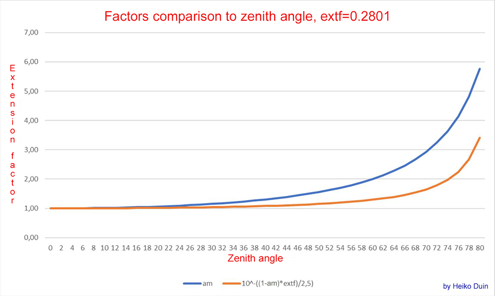
Source: Heiko Duin, Bremen
Illustration of the difference between the two airmass methods.
The blue line shows the course of the expansion factor when the horizon
brightens at the observatory (practically),
the orange line shows the extension factor without horizon brightening (scientifically).
The extf-0.2801 value corresponds to an
extf at sea level. (see
Reference, Table 1a)
Explanations about Airmass and Extinction (by Heiko Duin):
Extinction is given as a coefficient per airmass in magnitudes,
so the extinction for an object with an angle z from the zenith is:
airmass * ext_factor, where airmass depends on z.
Extinction depends on many factors, e.g. humidity and altitude above sea level
and is therefore difficult to calculate directly for a given location and
weather conditions.
Fortunately, the HORIZONS interface also provides Airmass and Extinction in the
ephemerides (a_mass and mag_ex).
These are determined according to the Obs code, so we don't have to worry about
altitude above sea level.
From the HORIZONS data you can easily determine the extinction coefficient with
extf = mag_ex / a_mass (in mag).
The reference measurement from K87 resulted in a specific magnitude for an
object.
However, in photometry the measured value is calculated to be �above the
atmosphere�.
This means that (at least) one airmass was already taken into account when
measuring on K87.
Therefore, only (Airmass � 1) needs to be taken into account when calculating
the extension factor.
If you now convert mag into flux and put everything together, you get the
extension factor vlf:
vlf = 10^((am-1)*extf/2.5) = 10^-((1-am)*extf/2.5)
am = airmass
This corresponds to the orange curve in the diagram, while the blue curve
indicates the associated airmass.
The extinction coefficient value of 0.28 comes from Green (1992) (http://www.icq.eps.harvard.edu/ICQExtinct.html)
and is an average extinction coefficient for a site on normal Zero level.
Light pollution does not affect extinction, at least I haven't found any
evidence of it.
The extension due to light pollution is controlled by the background value (in
mag per square arcsecond).
Reference: Green D. W. E. Correcting for Atmospheric Extinction, July 1992
Taking the Lunar Sky Brightness into account (all objects)
When the checkbox is activated, the Sky brightness due to moonlight and the
position of the object in the sky
is taken into account when calculating the number of images per group/stack.
The value is determined from the JPL HORIZONS API, here is the description:
Sky brightness due to moonlight scattering by Earth's atmosphere at the target's
position in the sky.
Output only for topocentric Earth observers when both the Moon and target are
above
the local horizon and the Sun is in astronomical twilight (or further) below the
horizon.
Galactic brightness, local sky light-pollution and weather are NOT considered.
Lunar opposition surge is considered. The value returned is accurate under ideal
conditions
at the approximately 8-23% level, so is a useful but not definitive value.
Source: Description
HORIZONS API
Quantity 48
Sky brightness due to moonlight is used together with the airmass value if the
checkboxes of both values are activated.
Both values are gradually integrated, otherwise only the activated value or
none.
The lunar sky brightness is multiplied by the number of
calculated images per group/stack using floating point
numbers.
Thus, the total number of images is increased during planning.
The calculation of the number of images including airmass and lunar sky
brightness is carried out using floating point numbers.
This means that it is not always possible to derive the number per group/stack
in Revise. Please take this fact into account!
The more images per group are originally required, the more accurate the result
will be.
If activated, it is no longer necessary to increase the groups in Revise in disturbing moonlight.